Data Validation Using Double Dependent Dropdown List – LibreOffice Calc

This tutorial will explain how to create a dependent dropdown list in LibreOffice Calc.

The earlier article explains a single dropdown list with data populated from a range inside the sheet. If you are new to dropdown lists data validation, you may read this first.

Data Setup

Say we have two lists containing values of their respective categories like this.

• Colors
  Orange
  Blue
  Black
  White
  Green
• Planets
  Pluto
  Mars
  Earth
  Venus
  Jupiter

We will have the first dropdown, which lists the categories, i.e. Colors and Planets.

Based on what the user chooses in the first dropdown, we want to fill the second dropdown with the list of items of the respective chosen dropdown.

I.e. If you choose Planets, the second dropdown would show a list of planets instead of a list of colours and vice versa.

Steps for Data Validation Using Double Dependent Dropdown List

• Select the categories, i.e. A1 and B1. Then from the menu, select Sheet > Named ranges and expressions > Define.

• Put name as category1. Click Add. You can put any meaningful name you want.

• Likewise, select A2 to B6 and add the named range as category2.

• Select E1, and from the menu select Data -> Validity.
  In the validity window, choose Allow=Cell range and put category1 as Source. Press OK.

• Select E2, and from the menu select Data -> Validity.
  In the validity window, choose Allow=Cell range and put below formula as source, then press OK.

INDEX(category2,,MATCH(E1,category1,0))

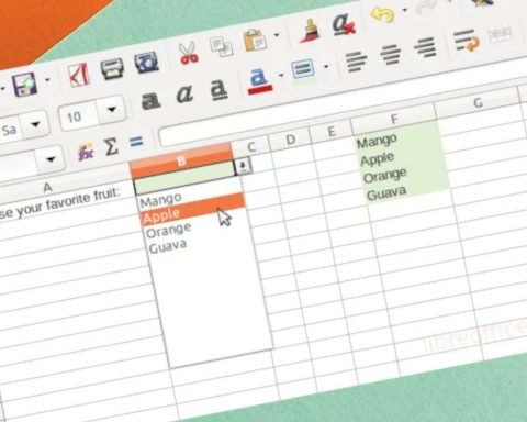
• Now, click on the small dropdown in E1 cell, you can see category1 i.e. colors and planets would be listed from A1:B1 cells.

• Select Planets.
• Now click E2 dropdown; you can see only planets values are loaded in this dropdown depending on the value of E1.

• Go back to E1 dropdown and select Colors. And likewise, open up the E2 dropdown. You can see it contains the color values dependent on the E1 value.

So this is how you can create a dependent dropdown in LibreOffice Calc.

Explanation of INDEX and MATCH in the second validation

INDEX(category2,,MATCH(E1,category1,0))

MATCH: It returns the relative position of the value selected in E1 after searching in category1 range (A1:B1). The last argument, 0 – denotes it would look for an exact match.

INDEX: returns the subset of an nXn range from reference category2 based on row and column number. The second argument is the row (which is omitted here as values are present in columns), and the third argument is the column number.

Learn more about Index and Match in this tutorial.

Watch this tutorial on Video

I have made the following video after many questions on Error 501 with the above instructions. The instructions are correct. Follow the steps exactly mentioned above.

Still, have questions? Drop a comment below.

Looking for something else?

Read our complete tutorial index of Calc, Writer, Impress and Draw.