The IF function is a powerful in-cell function in LibreOffice or OpenOffice Calc.
And you can do anything literally with it if you know the basics. Here’s how.
The basics are very simple. The IF function uses conditions to determine results. If the condition is met, then one result is shown, and if the condition is not met, then another result is shown.
Here are some examples to help you understand.
Table of Contents
IF Syntax
IF(Test, Then Value, Otherwise Value)
Simple IF Function examples
The below example checks whether the price is greater than $500, and based on that, we fill in High or Low in the adjacent cells.
=IF(A2>500,"High","Low")

The below example also gives the exact result. Note that the operator is changed to less than sign (<) and arguments have been swapped.
=IF(A2<500,"Low","High")

IF function usage notes
- You can use any comparison operators e.g. = (equal to), > (greater than), < (less than), >= (greater than or equal to), <= (less than or equal to) and <> (not equal to) in the IF formula.
- You can also use text/strings in IF statements with comparison operators. Remember to enclose the text or string using double quotes (“).
- The below example checks whether each cell contains ‘Mango’ then it returns ‘Fruit’ in the adjacent cell.

Nested IF examples
You can combine multiple IF statements for multiple conditions in a Calc cell. The FALSE or the third operator of the IF statement is replaced by another IF statement to evaluate another test or condition.
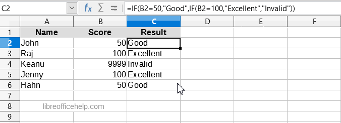
In the below example, if the score is 50, ‘Good’ is shown. If it is 100, then excellent; otherwise, it is invalid. You can note that all three possible tests are added in the single cell with two nested IF statements.
=IF(B2=50,"Good",IF(B2=100,"Excellent","Invalid"))
Conclusion
This is the most simple way to work in a Calc spreadsheet with conditions using IF. You can refer to the official guide here.
Drop a comment below if you have any questions.


hello. how can i compare two cells with date and time formatting to get the result in: morning or afternoon or evening.
I know I should use if, but and don’t know the logical terms. If it would be only time, i think it will be simpler, but time is together with the date, even the last one is not important for the result.
You can easily do it via – below. Say you have two times in cell A2 and A3: 12AM and 12PM. And you want to check input in C1 as 11AM. The formula would be as below.
“IF(AND(C1>A2,C1 A3),good morning,good afternoon)”
You can improvise with your needs.
This simple expression in a cell C1 of a new .ods document latest libre office 64 bit and one of its predecessors:
=IF(A1>0, A1,0)
(A1=1,B2=2,C1=expression)
causes error 509 (missing operator)
So condition is not working.
I dont wanna know what detail or secret is wrong, such things should not fail.
Sorry,
the statement is in the user language.
You can disable this in the settings or use if in your language, then it works.
I want to spectify the value of a cell like this:
IF(e3<g3,g3=e3)
In other words: I want to set cell g3 to the value of cell e3, in case e3 is less than g3. How can I do that?
Thanks for any hints
H. Stoellinger
Hello and thanks for the idea
My genealogical problem is I have a list of 9000 dna ‘relatives’
I want to identify those with a certain value over 90
=IF(G5>=90,”cousin”)
This does the trick, good
However, how do I find these “cousin” values?
If I do a find search it returns all the 9000 formula with cousin in them?
Is there a better way to do this rather than endless scrolling and wrist ache 🙂
Shay
You can refer to a Cell that contains “cousin”. =IF(G5>=90,”cousin”) can be changed with =IF(G5>=90,A1) where A1 will have cousin.
Also, if you are running this in a single cell, you can drag the cell handle for entire sheet. That way it can work.
If cell A contains the text “E” (between lets say E1, E2,E3 etc) then cell B=cell A. How can I do that with if function? Thanks in advance!
You can do this way.
=IF(AND(B1=A1,MID(A1,1,1)=”E”),”match”,”not match”)
Hello, My IF formula does not return expected results. In the following example, I want the results to be the value in col B IF the corresponding value in col C is blank; else I want the value to be blank. Example: Row 1 & 2 should return a blank. Row 3 should return 2500. The formula I came up with returns a blank for all 3 rows: IF(C3=” “,(IF(B3>0,B3)),” “). Where did I go wrong?
A ……B ……..C
1 ………………x
2 ………………x
3 …2500
This does NOT work for me!
I need to use ; instead of , for the IF formula to work.
I have been using COUNTIF in some analysis of weather data. Of course, it does a great job in determining how many days had daily high temperatures of, say, 100F or greater.
Can you suggest a way to count ‘streak’ data, i.e, how many days-in-a-row was that 100F temperature was achieved?
D’oh! After a little thought, this was a lot simpler to solve than I had originally anticipated.
I entered in the first cell, =IF(B4>=100,1,0).
I entered in the second cell, =IF(B5>=100,E4+1,0),
and dragged that cell down the column.
I want to add the contents of a cell to second cell only if a third cell contains an “*”. How do I format the proper IF statement in LiberOffice Calc? This is what I tried: IF( F3 =*,F26=(F26+E3),F26=F26).
if cell have any character (alphabet or numeric or symbol) then value it 2 otherwise 0