Find the last position of a character in LibreOffice Calc easily using various methods in this comprehensive guide.
In today’s fast-paced business world, efficiency is key, and one of the ways to streamline processes is by using the LibreOffice spreadsheet program. LibreOffice and its powerful components allow users to manipulate, organize and analyze data in various ways.
In this article, we will cover various methods to find the last position of a character in LibreOffice Calc, which is considered one of the common problems while working with spreadsheets.
The following methods use common functions such as LEN, FIND, SUBSTITUTE, and others to get the result.
Table of Contents
Find the last occurrence of a character in LibreOffice Calc
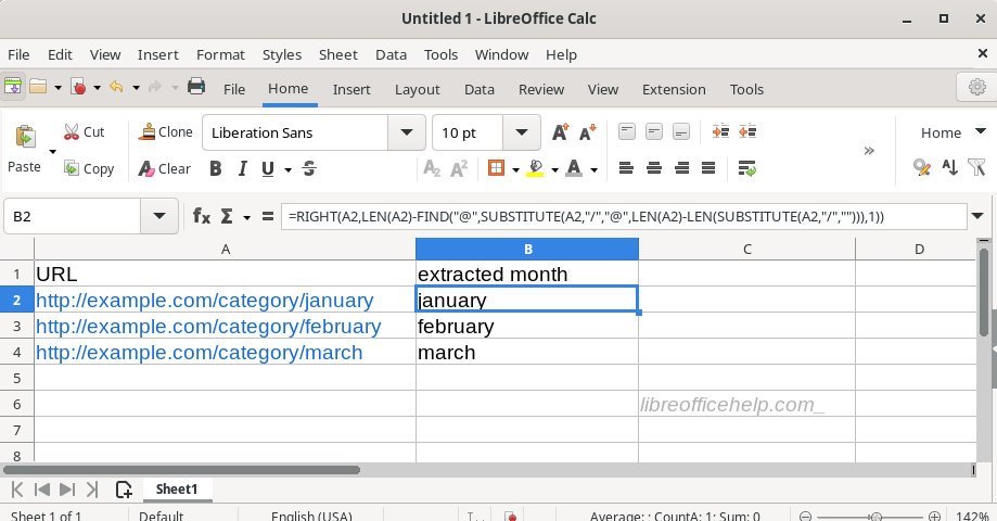
Let’s explain this with an example. I have the following list of web URLs. As you know, the URLs contain several forward slashes “/”. In this example, the last section of the URL is the month. So, if I want to extract the month portion of the URL, then I need to find out the last occurrence of the forward slash character.
| URL | extracted month |
| http://example.com/category/january | january |
| http://example.com/category/february | february |
| http://example.com/category/march | march |
To do that, I will use this formula which I put in a new column.
=RIGHT(A2;LEN(A2)-FIND("@";SUBSTITUTE(A2;"/";"@";LEN(A2)-LEN(SUBSTITUTE(A2;"/";"")));1))
And drag the cell handle down to fill it up till the last row of data. And you can see the month portion is separated as a result.
But how does this formula work?
Let’s explain by the last section of the formula.
SUBSTITUTE(A2;"/";""): This substitute function replaces the forward slash with an empty string. So, if you are trying to find any other character occurrence, use it here instead of the forward slash. The output of this piece is below for the first cell A2:
http:example.comcategoryjanuary
LEN(A2)-LEN(SUBSTITUTE(A2,"/","")): Now, we need to calculate the length of the entire URL without the forward slash. And then subtract it from the entire length with the forward slash. This will give you the effective count of total forward slashes in the URL. In this example, for cell A2, it would be 4.
35-31=4
SUBSTITUTE(A2,"/","@",LEN(A2)-LEN(SUBSTITUTE(A2,"/",""))): The substitute function can replace a specific occurrence of a character with any other character. The last argument is the occurrence number of this function. Applying this principle, this part of the formula replaces the 4th occurrence of the forward slash (the last one) with any unique character, such as “@”. You can use any other character you want, make sure it doesn’t appear as part of the URL. So the result of this would be below:
http://example.com/category@january
FIND("@",SUBSTITUTE(A2,"/","@",LEN(A2)-LEN(SUBSTITUTE(A2,"/",""))),1): So, you have the position identified with the character “@”, and all you need to do is use the FIND function to find out its position. The result is 28.
LEN(A2)-FIND("@",SUBSTITUTE(A2,"/","@",LEN(A2)-LEN(SUBSTITUTE(A2,"/",""))),1): If you subtract it from the entire length of the A2, you get the actual starting position of the string “january”.
7
Finally, use the RIGHT function to extract the past portion of the URL text from the right side.
=RIGHT(A2,LEN(A2)-FIND("@",SUBSTITUTE(A2,"/","@",LEN(A2)-LEN(SUBSTITUTE(A2,"/",""))),1))
So, effectively the above function translates to:
=RIGHT(A2,7) // returns January
Find the first or nth occurrence of character with the formula
Using the above principle, you can find out the first occurrence or nth occurrence of a character in a LibreOffice Calc cell string in the most easiest way.
To find the first occurrence, use this formula:
=FIND("@",SUBSTITUTE(A2,"/","@",1))
Explanation: The first position number is mentioned as 1 at the end. The forward slash is the character you want to find. And “@” is any character which is used for temporary calculation and should not be part of the source text.
To find any position, such as the nth position, you can simply replace the 1 with any position number you want. For example, if I want to find out the position of the 3rd occurrence of a forward slash in the above example, I would use below:
=FIND("@",SUBSTITUTE(A2,"/","@",3))
And that’s it.
Closing Notes
In conclusion, finding the last position of a character in LibreOffice Calc can be achieved through various methods, from simple to advanced techniques. Whether you are a beginner or an experienced user, you now have the knowledge and skills to find the last position of a character in Calc with ease and confidence.
You can now apply the above learning for any use cases.
Cheers.

Perfect tutorial. I needed to cut off last three comma separated parts of a string and concat them with another string. Super useful explanations here!
Thank you very much.