This article explains how you can do a case-sensitive lookup in LibreOffice with some examples.
In the prior articles, we have explained the concept of lookups with VLOOKUP, INDEX and MATCH. Together, they can be a great way to achieve several filtering results.
However, most of them are not case sensitive. That means if you search for lowercase data in cells, it searches for lowercase and uppercase.
Hence, it’s important for you to learn the case sensitive lookups. Here’s how.
Table of Contents
Case sensitive lookups with examples
It’s easier to understand using an example.
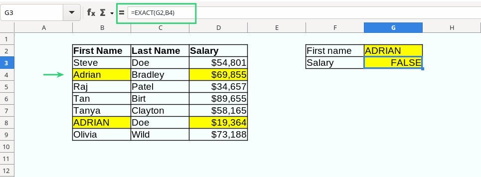
We have the following set of data on employees and their salaries. In cells B4 and B8, we have the same name but with different cases i.e. “Adrian” and “ADRIAN”. The goal is to find out the correct salary based on the case of the search key on G2.

LibreOffice does not have a built-in function for performing case-sensitive lookups. However, you can combine the MATCH and EXACT functions to achieve this.
EXACT Function
The EXACT function matches two texts accordingly to the case and returns TRUE or 1 if they matches and FALSE or 0 if they don’t match.
Syntax
EXACT(text1, text2) : returns TRUE if both matches with case, otherwise FALSE
If you apply the EXACT function in the above example with B4, then it should return FALSE.
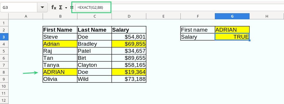
Similarly, when you use the EXACT function with cell B8, it should return as TRUE.
Since we have a set of data to be searched, we will apply the array formula of LibreOffice Calc. The array formula searches for a value in a set of values instead of a single cell.
Find the row of the case sensitive match
The primary objective is to search for “ADRIAN” in all the cells from B3 to B9. And get the return row number. As you can see above, the ADRIAN is present at B8, i.e. row 6 of the selection B3:B9.
To apply the array function, we need to search for the TRUE (i.e. which matches by case) via the MATCH function.
{=MATCH(1,EXACT(G2,$B$3:$B$9),0)}
Insert the above formula and press CTRL+SHIFT+ENTER to make it an array formula. You should see the formula is enclosed by {} , i.e. it is converted to an array formula. Don’t enter {} manually.
Explanation: The above EXACT array function returns an array like this: {FALSE,FALSE,FALSE,FALSE,FALSE,TRUE,FALSE}. The key value of MATCH, which is 1 or TRUE, is searched inside the return values and returns the 6th position where ADRIAN matches.

Find the final result
As you can see, now you have the row of the search key, it’s now easy to find out the Salary via a column search via INDEX. The INDEX function returns a cell based on row and column.
{=INDEX($D$3:$D$9,MATCH(1,EXACT(G2,$B$3:$B$9),0),1)}
Explanation: The above INDEX function returns the salary from column D3:D9 at position 6 and column 1 (since we have selected only one column). The position 6 is already returned via the MATCH and EXACT combination above.
And here’s the final output.

Wrapping Up
I hope this tutorial helps you to understand the concept of case sensitive lookup in LibreOffice and how it can be done via several combinations of functions. You can extend this concept to more complex use cases for your need.
Have a question? Let us know in the comment box.