This is how you can fix the Calc spreadsheet err 502.
If you are an avid user of spreadsheet programs such as Excel, Calc in OpenOffice or LibreOffice, you might have encountered the Err:502 while performing calculations using functions. Here’s how you can fix it.
Table of Contents
What is Err 502
As the Calc manual says – it occurs when – “A function argument has an invalid value or invalid function argument”. It can happen to any function if you pass invalid arguments it was not supposed to receive.
How to fix Err 502
A typical way to fix this error is – to check each and every function and its parameters which you are passing. Likely you are providing some incorrect argument that is causing this error.
See some examples below.
Examples
- If you pass a negative number to SQRT (square root) function – Error 502 will be thrown by Calc. Because it expects a positive number, and you are passing a negative.
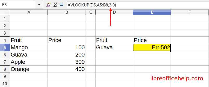
- If you are using VLOOKUP and trying to return some value from the column, but the column number doesn’t exist in the selected table, you will get Error 502.
Conclusion
Almost all functions can return Error 502 if you pass an invalid argument. Carefully checking your spreadsheet to find out about the error and assessing the arguments is the recommended way to solve this problem.
Summary
Time needed: 5 minutes
How to fix Error 502 in Calc
- Select the Cell in Calc which contains the Err 502
Select the cell
- Analyze the function
Analyze the argument of the functions or functions (in the case of nested formula) and change the arguments.
- Run your formula
Recalculate Calc formula to eliminate Err 502.
Are you facing the Error 502 problem and unable to solve it? Drop a comment below for help.

I’m getting a 502 error but only for data from the 14th column and after. All data in columns 1-13 works perfectly. Is there a limit to the number of columns VLOOKUP will handle?
There is no limit for number of columns in VLOOKUP. Check your source array and column numbering.
Ok, someone on another message board I’m on figured it out. Evidently, the “M” refers to the last column looked at by VLOOKUP. As I was trying to pull data from beyond that column, that’s what was causing the error.
I changed “M” to “Z” and the problem is now solved.
Huh… I honestly don’t see anything “wrong” with it. I’ve literally copy-n-pasted the VLOOKUP argument so I know it’s identical, except for the column from which it’s pulling that cell’s requested data.
Here’s what I’ve got:
=IF(H6=0,"",(VLOOKUP(H6,$'Data Lookup'.A:$'Data Lookup'.M,14,0)))Everything stating M.13.0 and less (down to M.2.0, since M.1.0 is the initial search criterion) works perfectly. Just 14 and up do not work and return the 502 error.
This spreadsheet has six sheets to it.
The first sheet is a data entry sheet, where I type in the store number (along with first day of that week and team members I’m working with), and it’s broken out to give me five days, and then these are grouped into four groups (i.e. four weeks).
The second, third, fourth, and fifth sheets are weekly result tables which I can print.
The sixth sheet is the Data Lookup sheet, and it’s a massive table of store numbers (first field) and then all the other pertinent data for each of those stores (district, phone number, address, and so on).
I don’t understand. I’m getting this error.
I have a cell with “00:47:05” in it. It’s in position B5. When I do the function “=TIMEVALUE(B5)” I get error 502, but when I do the function “=TIMEVALUE(“00:47:05″)” I get the converted value.
I cannot seriously be expected not to use a cell within a function in a spreadsheet program. Hell, I have seen such being described here. Something is wrong, and I don’t know what it is.
Hi, I am trying to apply the command minverse in calc and I get a 502 error. When an error 502 may exist in this specific command?
I am puzzled by this error in COUNTIFS() function. It is said to accept arbitrary number of argument pairs but in fact accepts only two pairs, as in the tip shown on yellow when typing the formula. Why is it so? Am I missing something?
Thanks for the great article anyway.
Some argument is incorrect in COUNTIF(). Check this article.
https://www.libreofficehelp.com/count-cells-strings-numbers-countif-function-calc-example/
Why Error # 502 “Invalid argument” ?
This is the formula for cell F9:
=INDEX(category,MATCH(B9,pounds,0),MATCH(E9,bminumber,0))
According to: LibreOffice 7.0 online help,
INDEX(Reference [; Row [; Column [; Range]]])
INDEX only requires Reference which in above formula is category.
MATCH(SearchCriterion; LookupArray [; Type])
SearchCriterion: B9 & E9 , LookupArray: pounds & bminumber, Type: 0 exact match
I have also tried this formula for cell F9:
=IFERROR(INDEX(category,MATCH($B9,pounds,0),MATCH($E9,bmiumber,0)),””)
This formula does not trigger an error, but it also does not return any text from the help table as expected even when there is text in the help cell for that cross reference.
The value of cell B9 is entered by user. The value of E9 is derived by a formula. =ROUNDUP((B9*703)/INT($D$9*$D$9),0)
Something is definitely incorrect in the argument. Do this. Split your formula into separate cells. And see what they are returning before applying it to INDEX. Both of your MATCH formula – put in different cells and see if they are returning the desired result.
सही अनुमान इंगित करने वाला उदाहरण
correct guess example
Goal: get the value of the price of a property that precedes the address as text:
example: if cell A2=
599,630 0 Robert White Rd 122; (where 599,630 is the price)
using (=value(left(A2;9) results in Err:502.
What is needed is an “If” statement to handle the Err result (such as If(ERRORTYPE()=502…….??
I have tried several methods but still need a solution. Thanks
Because VALUE() can’t convert a space to a number. In your example, the 8th position from left is a space. Hence the error. If you use only 7 digits, it should work:
Im trying to vlookup and getting an error. This is the first time im using Libre office.
Replace 5 with 3. In your selected table the 3rd column is the amount.
=VLOOKUP(H2,$C$2:$E$7,3,0)
Read more about VLOOKUP here: https://www.libreofficehelp.com/vlookup-libreoffice-calc/
I did that and got this
This is the selection
I am trying to either return the numbers in a column that has all cells with text results; with the formula :=IF(VALUE(D30)>0.1;VALUE(D30);””): every third cell will return the number -value of the text, but the next two cells return “Err:502”. I am trying to get the sum of the cells that actually return numbers. (The “If” function does not return “”)