


This tutorial would explain how to Freeze, Unfreeze rows and columns, and ranges in LibreOffice calc.
There are different display devices, and monitors available with various sizes and resolutions. When you are working with a spreadsheet and doing data analysis, it is often needed to freeze certain rows and columns while the rest of the section of the spreadsheet can move using scroll bars. Here’s how you can do it in LibreOffice Calc:
Freeze rows and columns together
Select a cell. (In this example C6).

Go to the menu and select View > Freeze Rows and Columns. if you are using Tabbed UI of LibreOffice, go to the View tab and click on “Freeze rows and columns”.
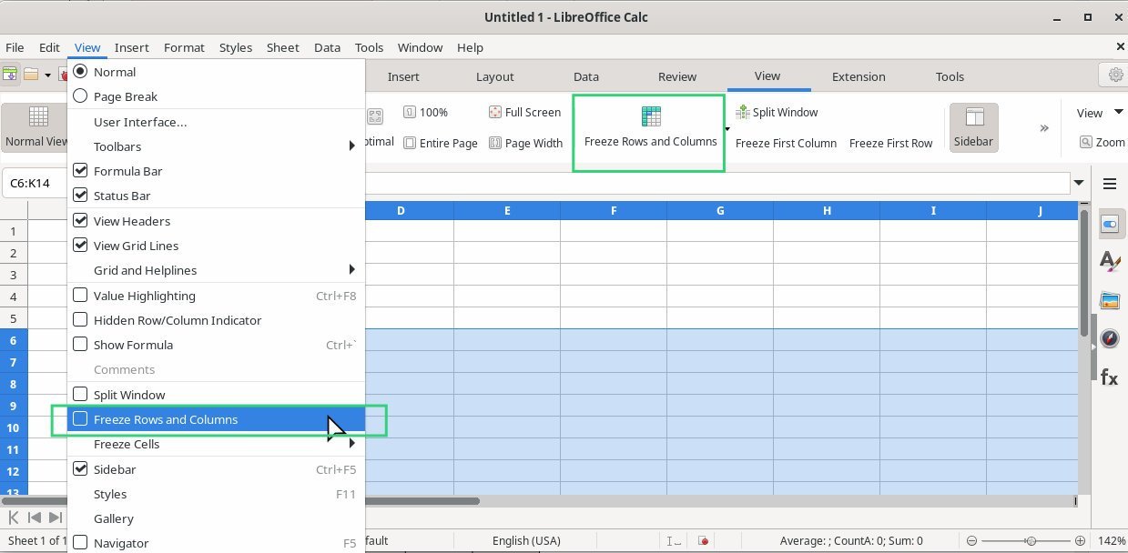
LibreOffice Calc would freeze all the sections left and top of the selection, which is C6 in this example. the freeze section should be marked with a thick border as you can see in the below image.
So, if you scroll vertically or horizontally. And the range A1:B5 would remain fixed while the rest of the sheet’s content can move.

You can also quickly use options Freeze first row and first column to freeze the first row and column respectively.
Unfreeze
To unfreeze, use the option Unfreeze from the menu.
There is no unfreeze option in the menu of LibreOffice Calc. To unfreeze, follow the below steps:
- Select/click any of the cells inside the frozen row/column range.
- Go to Menu and click on View > Freeze Rows and Columns again.
This will remove all ‘freeze’ from the Calc sheet.