A comprehensive article to understand VLOOKUP in LibreOffice Calc spreadsheet program.
VLOOKUP is a kind of search/lookup function in LibreOffice Calc or any popular spreadsheet program such as Microsoft Excel. It’s an abbreviation of “vertical lookup” and searches vertically, i.e. Top to bottom in a table, hence the name.
In a nutshell, the function searches your key to a list/table and returns a value associated with that matched value.
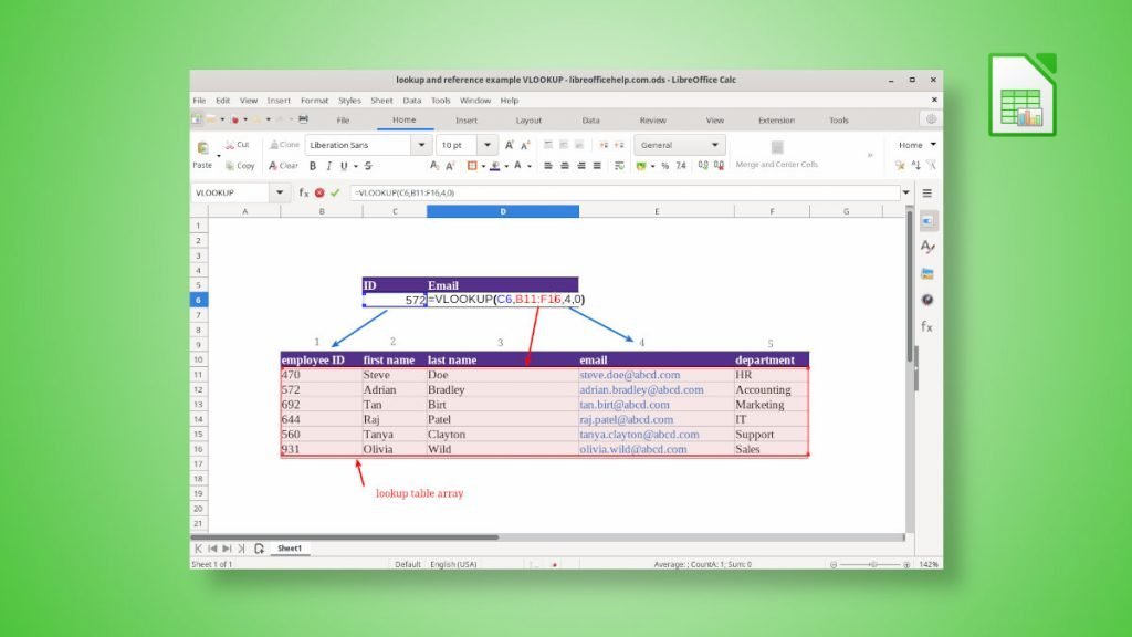
For example, I have the following data set of employees of an organization. How can I find the email address of a specific ID in this table?
Let’s find out.
Table of Contents
VLOOKUP in LibreOffice Calc
Syntax of VLOOKUP
=VLOOKUP(search_key, table_array, column number of table array to be returned, search_type)
search_key: the value you want to search for
table_array: where you want to search
column number: if found which column of value you want to return
search_type: 0=Exact match; 1=Approximate match; default is 1 (approx match).
Example
In the above example, if I need to find out the email address of Adrian whose ID is 572; I should use the following formula:
=VLOOKUP(C6,B11:F16,4,0)
Explanation: The above formula searches C6, i.e. 572 in the range B11:F16, and returns column # 4 from the range. The match type is a EXACT match. Hence the value is zero.
Here’s a detailed explanation in an image.
Since you understand the basics, let’s learn some important aspects of VLOOKUP.
An absolute and relative reference in VLOOKUP
In the above example, you can see the range reference is used as B11:F16. This is called a relative reference.
But there is a problem here.
If you search a set of values with relative reference and drag the cell handle to fill up the rest of the rows, then B11:F16 gets incremented. That is, the following search happens with B12:F17.
That’s not good if the table_array is changing for each key value.
So, always use the absolute reference with the $ sign or press F4 to convert it. Finally, the proper formula becomes this.
=VLOOKUP(C6,$B$11:$F$16,4,0)
Learn more about the relative and absolute references in this guide, which I explained in detail.
VLOOKUP only look at the right
At the backend, the function always searches to the right, starting from the top. So, you should keep this in mind while preparing your data or writing the function. Here’s how you can visualize the general workflow of VLOOKUP.
The key should always be the first column in the table array
One of the important aspects of VLOOKUP is the key field. The first column of the search table (table_array) should always contain the values of your key field.
For the above example, if your ID field appears after Email or Name, then VLOOKUP will not work.
Approximate and exact match
The fourth parameter of VLOOKUP is wither TRUE or FALSE. This denotes the following.
- 0 or FALSE: Exact match, i.e. entire string should match and values returned
- 1 or TRUE: Approximate match
Let’s consider the following example, where I am searching for commission % for a range of sales figures.
If I want to find out the commission for the sales amount 550 $? Because 550 is not present in the table!
Here, you need the approximate match, i.e. the final argument as 1.
So, if I put a formula as below, I can get the commission 11% for $550.
=VLOOKUP(C6,C11:D16,2,1)
Explanation: VLOOKUP tries to find out whether there is an exact match present for 550. And it’s not present in the table. As a next step, it tries to go a step back and returns the closest match, which is 544. And finally returns the 11%.
Here are a couple of things you should remember here:
- When using an approximate match, ensure the key column table_array is sorted.
- The sorting order should be ascending.
- If it’s not sorted, then VLOOKUP may give you a #N/A error or incorrect result.
- This parameter is optional. If you omit this in VLOOKUP, then the default is taken as 1, i.e. approximate match.
So, use this approximate match with caution.
VLOOKUP only returns the first match
As you can see in the above example, only the first one is returned when there are two values of the approximate match.
This also applies to the exact match as well.
In the first example, if I change the last name of Steve to Patel and try an exact match, what should VLOOKUP return?
=VLOOKUP(C6,$D$11:$E$16,2,0)
As you can see, there are two matches as highlighted below. In this scenario, VLOOKUP returns the first exact match.
Wildcard match in VLOOKUP
VLOOKUP in LibreOffice Calc also allows wildcard search with “*” (Asterix). You can specify the “*” in search_key. When you use a wildcard, remember you should always use the exact match type, i.e. FALSE, as the final argument.
=VLOOKUP("Pate" & "*",$D$11:$E$16,2,0)
So, if you use the above formula, it returns the exact same result as the previous example.
VLOOKUP and #N/A errors in LibreOffice Calc
If you use this function, for sure, you will run into #N/A error as a result of VLOOKUP. The #N/A means the match is not found.
If you are unable to solve #N/A error, here are some of the reasons you should know.
- The search_key or look-up value is not present in the table (first column of table_array).
- The search_key may be misspelt or may contain extra space. You might want to remove space using trim function.
- Carefully check the search_type to see whether you have specified Exact or Approximate
- The table_array is not correctly mentioned. Be careful whether it is locked with relative reference or abosulte reference.
Wrapping Up
In this article, you learned how you could easily perform VLOOKUP in LibreOffice Calc cell. It is one of the powerful functions which can do anything if used properly. If you run into an error or have any questions, let me know in the comment box below.

